6. PreREISE
This page is dedicated to the collection, processing and formatting of data that are fed to the simulation engine. PreREISE is an open source package written in Python that is available on GitHub.
The generation of input data rely on the grid model. For this reason, you must have PowerSimData cloned in a folder adjacent to your clone of PreREISE.
Note
Input data are publicly available for the Breakthrough Energy Sciences (BES) grid model (see publication). You don’t need to generate any input data if you use the scenario framework to carry out power flow study.
6.1. General Comments
Profiles are CSV (Comma Separated Values) files enclosing a series of data points indexed in time orders. The simulation engine expects a demand, hydro, solar and wind profile. All the profiles have UTC timestamp as indices. Columns are the zone IDs and plant IDs for the demand and hydro/solar/wind profiles, respectively. Values are load in MWh in each zone for the demand and energy generated by a 1MW generator for hydro, solar and wind profiles.
The [type]_v[D] naming convention is used, where:
type specifies the profile type (demand, hydro, solar or wind) and
D refers to the date the file has been created using the 3 letters Month (e.g., Jan) and 4 digits Year (e.g., 2021) format.
If two or more profiles of the same type are created the same month of the same year,
the different versions will be differentiated using a lowercase letter added right
after the year, e.g, demand_vJan2021.csv (first), demand_vJan2021b.csv (second),
demand_vJan2021c.csv (third) and so forth.
6.2. Demand
6.2.1. Historical
6.2.1.1. Texas
ERCOT publishes historical hourly load data for its eight weather zones. The data downloaded here are used as is to build the profile for the Texas Interconnection.
6.2.1.2. Western
Balancing authorities (BAs) submit their demand data to EIA and can be downloaded using an API. The list of BAs in the Western Interconnection can be found on the website of the Western Electricity Coordinating Council (WECC) along with the area they approximately cover (see map).
Some data processing/cleaning is then carried out to derive the profile for the Western Interconnection:
adjacent data are used to fill out missing values
BAs are aggregated into the load zones of the grid model
outliers are detected and fixed.
These steps are illustrated in the western demand notebook.
6.2.1.3. Eastern
The construction of the Eastern Interconnection demand profile is slightly different from the Western counterpart. We still download historical demand data from EIA and perform the 3-step data processing/cleaning as for the Western Interconnection for all Balancing Authorities (BAs) but MISO (Midcontinent Independent System Operator) and SPP (Southwest Power Pool).
MISO and SPP operate across multiple U.S. states (e.g. 15 for MISO) and cover several load zones in our grid model. Instead of considering a single hourly profile shape for each entity and having load zones sharing the exact same profile in different part of the country, we further split MISO and SPP into subareas. The hourly subarea demand profiles for MISO and SPP can be downloaded on their respective website (check SPP hourly load and MISO hourly load). The geographical definitions of these subareas are obtained directly from contact at the BAs via either customer service or internal request management system (see the RMS for SPP). Given the geographical definitions, i.e., list of counties for each subarea, each bus within MISO and SPP is mapped to the subarea it belongs to.
The overall procedure is is demonstrated in the eastern demand notebook.
6.2.2. Transportation Electrification
6.2.2.1. Summary
Decarbonizing the transportation sector is one of the five grand challenges of decarbonizing the economy. In order to accurately capture the future trend of transportation electrification and its interactions with the electricity sector and other sectors such as building and manufacturing, a high resolution and accurate transportation electrification model integrated into the simulation framework with other sectors is necessary. A few key questions arise when determining the additional load from charging electric vehicles on the electric grid – how many electric vehicles of which types are expected to be on the roads by a given year and what are their typical trip patterns, which in turn determines when charging is most likely to happen. As is frequently discussed, charging could have significant flexibility as to its precise timing, which ties this project into the Demand Flexibility project. In future, highly integrated whole-economy energy systems, the optimal operation of the transportation sector is affected by other sectors, such as the building sector. When electric vehicles are charged through chargers located in buildings, the distributed energy resources and space heating/cooling load in buildings could be optimized together with electric vehicle charging to achieve more emissions reduction and cost savings. This transportation model is one of the key components of the multi-sector integrated energy systems model.
The overall objective of the Transportation Electrification Project is to develop a module that can capture the magnitude and spatiotemporal variation of the additional electricity demand from electrification of most of the on-road transportation sector, including electric light-duty vehicles (LDVs), light-duty trucks (LDTs), medium-duty vehicles (MDVs), and heavy-duty vehicles (HDVs), including fleet vehicles (e.g., buses). The core activities include (1) development of detailed data sets that represent the electricity demand patterns due to vehicle mobility, growth in electric vehicle penetration, and flexibility parameters for electrified LDVs, LDTs, MDVs, and HDVs consisting of private and publicly-owned fleets; (2) development of code that can generate electricity demand profiles for each vehicle type under different levels of charging intelligence; and (3) integration of the modeling capability for determining electrified vehicle load profiles into the open-access, large-scale grid model developed by the Breakthrough Energy Grid Modeling team.
6.2.2.2. Capabilities and Data
The transportation electrification module calculates an estimate of the additional hourly electricity demand from the electrification of transportation vehicles for all U.S. urban and rural areas for years ranging from 2017-2050. The hourly estimation builds upon data collected representing over half a million driving events.
Additional data sets allow for profiles to be generated across the following dimensions:
4 vehicle types (LDV, LDT, MDV, and HDV)
34 simulation years (2017-2050)
481 Urban Areas (as defined by the U.S. Census Bureau) and 48 Rural Areas (one for each continental U.S. State).
The charging of each vehicle is currently simulated via one of two methods: Immediate Charging and Smart Charging.Immediate Charging simulates charging occurring from the time the vehicle plugs in until either the battery is full or until the vehicle departs on the next trip. An example profile is in orange below, added on top of an example of non-transportation base demand (Fig. 6.1).
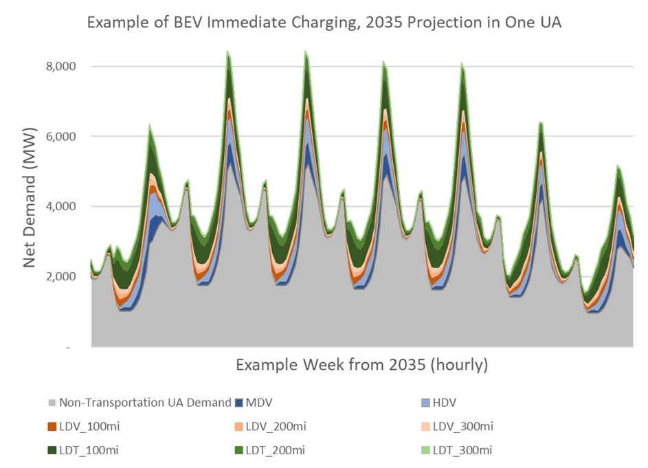
Fig. 6.1 Example of BEV Immediate Charging stacked on top of non-transportation base demand
Smart Charging refers to coordinated charging between drivers (either in aggregate or individually) and utilities or balancing authorities in response to a user-adjustable objective function. The example profile below (Fig. 6.2) provides the same amount of charging energy to the same set of vehicles in the Immediate Charging figure above (Fig. 6.1). This instance of Smart Charging manages the peak demand of the non-transportation base demand plus the additional transportation electrification load to be substantially lower.
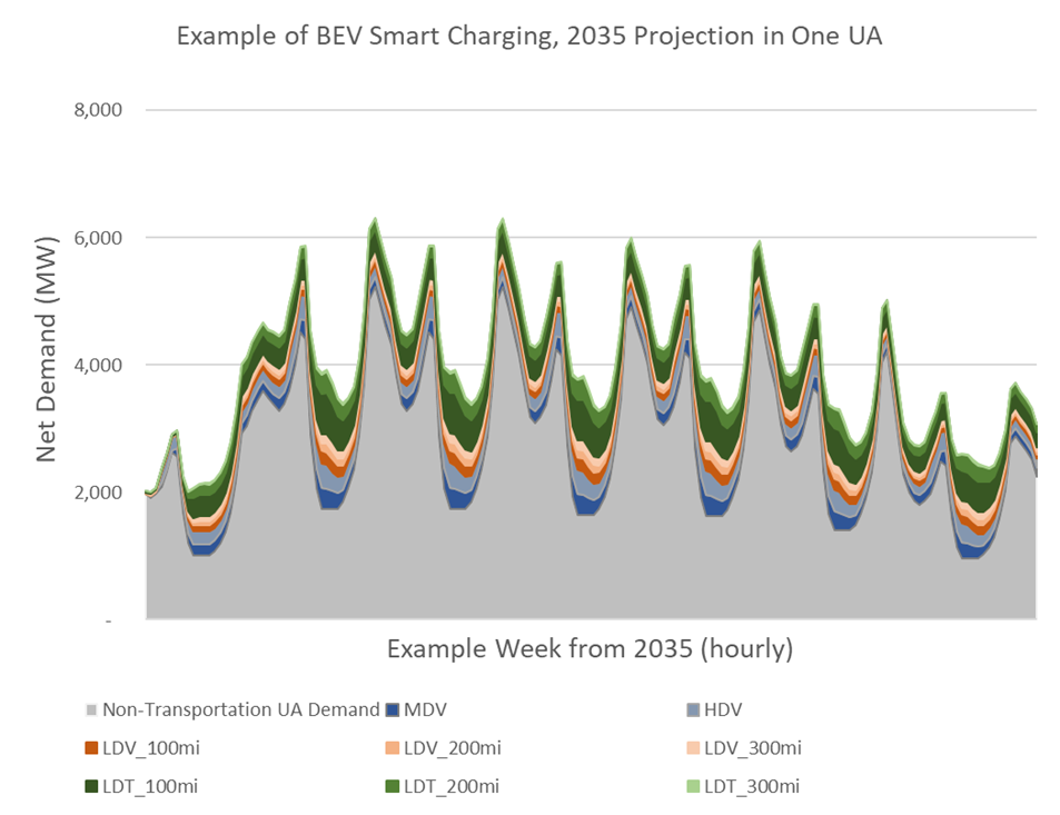
Fig. 6.2 Example of BEV Smart Charging “filling in the Valleys” of non-transportation base demand
6.2.2.3. User Manual
6.2.2.3.1. Pre-processed input data
The following data is provided for the user or could be overridden via an input from the user with a different preferred data set.
Annual projections of vehicle miles traveled (VMT) are calculated in advance and are provided for the user for all Urban Areas in the U.S. Each state also has a VMT projection for the Rural Area in that state. See Section Section 6.2.2.4.3.1 below for calculation process details using data from the National Renewable Energy Laboratory (NREL)’s Electrification Futures Study (EFS) and the Department of Transportation’s Transportation and Health Indicators.
Projections of the fuel efficiency of battery electric vehicles are provided from NREL’s EFS, with more detail in Section Section 6.2.2.4.3.4 below.
Each vehicle type (LDV, LDT, MDV, and HDV) has a dataset with vehicle trip patterns that is used by the algorithm to represent a typical day of driving. See Sections Section 6.2.2.4.1 and Section 6.2.2.4.2 for more details on the input data from the National Household Travel Survey (NHTS) and the Texas Commercial Vehicle Survey.
Each typical day of driving is scaled by data from the MOVES model from the U.S. Environmental Protection Agency (EPA) that captures the variation in typical driving behavior across (i) urban/rural areas, (ii) weekend/weekday patterns, and (iii) monthly driving behavior (e.g. more driving in the summer than the winter).
6.2.2.3.2. Calling the main Transportation Electrification method
With the above input data, the main function call for the transportation module is
prereise.gather.demanddata.transportation_electrification.generate_BEV_vehicle_profiles
and is called using a few user-specified inputs:
Charging Strategy (e.g. Immediate charging or Smart charging)
Vehicle type (LDV, LDT, MDV, HDV)
Vehicle range (whether 100, 200, or 300 miles on a single charge)
Model Year
U.S. State and the underlying Urban Area(s) / Rural Area that are being modelled
Depending on the spatial region included in the broader simulation, the user can run a script across multiple U.S. States to calculate the projected electricity demand from electrified transportation for the full spatial region. From there, a spatial translation mechanism (described next) converts this demand to the accompanying demand nodes in the base simulation grid.
6.2.2.3.3. Spatial translation mechanism – between any two different spatial resolutions
We have developed a module called prereise.utility.translate_zones. It takes
in the shape files of the two spatial resolutions that the user would like to transform
from one into the other. Then a transformation matrix that gives the fractions of every
region in one resolution onto each region in the other resolution will be generated
based on the overlay of the two shape files. Finally, the user can simply multiply
profiles in its original resolution, such as Urban Areas (UA) and Rural Areas (RA), by
the transformation matrix to obtain profiles in the resultant resolution, such as load
zones in the base simulation grid. This allows each module to be built in whatever
spatial resolution is best for that module and to then transform each module into a
common spatial resolution that is then used by the multi-sector integrated energy
systems model.
6.2.2.4. Methodology
6.2.2.4.1. EV Charging Model Process and Flowchart
This EV charging model simulates the charging behavior of the following on-road vehicle categories: LDV, LDT, MDV, and HDV. The default LDV and LDT trip data come from the 2017 NHTS, with an example of the data included in Fig. 6.3.
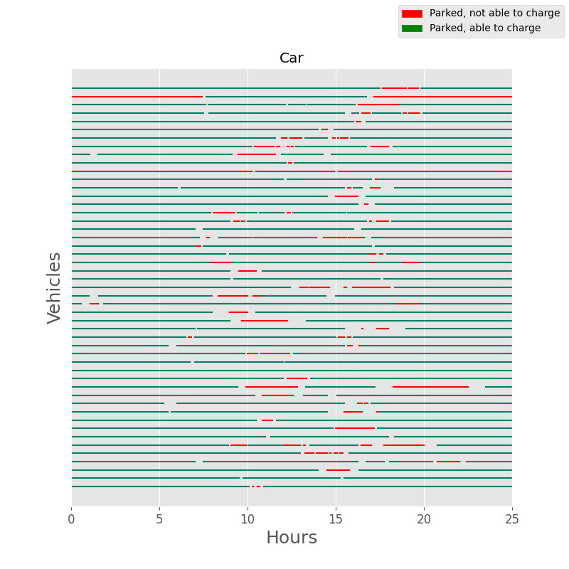
Fig. 6.3 Example daily trips of vehicle data from NHTS
These are also divided into Census Divisions, which are then mapped to the corresponding regions within the grid model. The MDV and HDV trip data are anonymized from the Texas Commercial Vehicle Survey and calibrated to align with medium- and heavy-duty vehicle trip statistics. More details about each data set are included in Section 6.2.2.4.2 and can be updated to reflect different vehicle scenarios or incorporate more recent data. In all cases, an average weekday and average weekend daily pattern of vehicle trips is calculated from the vehicle trip data. Then, these trips are filtered by vehicle type (e.g. LDV, LDT, MDV, and HDV) and by range for LDVs and LDTs (e.g. less than 100 miles, less than 200 miles, less than 300 miles) to capture what is capable for typical battery capacities. This creates a weekday and weekend daily pattern of BEV-capable trips that will be used in the subsequent steps. The LDV and LDT vehicle miles traveled (VMT) by hour is presented in Fig. 6.4.
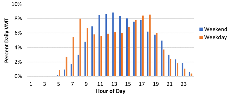
Fig. 6.4 Light-duty vehicle/truck miles traveled by hour of the day for weekends and weekdays
Similarly, Figure Fig. 6.5 illustrates the percentage of vehicles parked and able to charge at each hour over a 24-hour period.
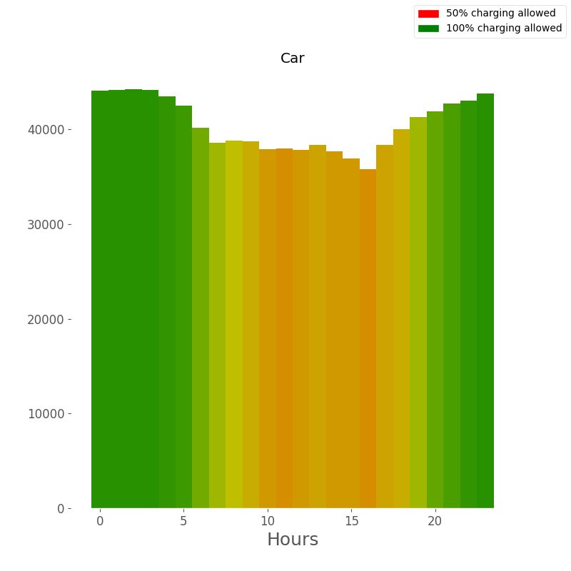
Fig. 6.5 Status of dwelling vehicles over 24-hour period
The flowchart in Fig. 6.6 illustrates the entire procedure.
Fig. 6.6 Workflow from input trip data to weekday and weekend trip patterns
These daily BEV-capable trip patterns are then further distributed temporally and spatially, as discussed in more detail in Section 6.2.2.4.3. State-level and UA VMT per capita were taken from the Department of Transportation’s transportation health tool and create the distribution across rural and urban areas, as defined by the U.S. Census Bureau [1], [2]. Weight factors from the U.S. EPA model, MOVES, create the time-of-year scaling of weekday versus weekend and month of the year [3].
Projections from NREL’s EFS provide the adoption rate scaling of BEV demand to create the base-year and simulation-year profiles of BEV-capable trip patterns [4]. Total charging demand by area (urban and rural) is scaled based on state-level BEV VMT projections from NREL’s EFS. As more granular BEV projections become available, scaling projections could be targeted to specific urban and rural areas given the model’s structure. The procedure is shown in Fig. 6.7.
Fig. 6.7 Workflow from weekday and weekend trip patterns to annual VMT pattern
Algorithmically, these projections are modeled by making multiple copies of individual trips, as illustrated in Fig. 6.8, which are used in the smart charging algorithm.
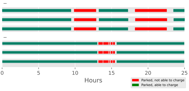
Fig. 6.8 Scaling process of vehicle trip
With the projected BEV vehicle trips in place, NREL’s EFS is again used to set the fuel efficiency for the simulated year to determine the amount of electricity needed to charge after each BEV trip. Then, the charging model uses one of two charging algorithm strategies: immediate (uncoordinated) charging and smart (optimal) charging, with example illustrations shown in Fig. 6.10 and Fig. 6.11. Both algorithms are deterministic and directly utilize the input vehicle trip data to calculate the charging demand based on vehicle travel distances, dwell locations, and user defined infrastructure parameters. The Smart Charging algorithm currently uses an optimization function to minimize wholesale prices via flattening the net load curve. Incorporating additional optimization goals that will change the cost function, such as minimizing individual vehicle costs in response to time-varying utility rate structures, could be explored in future work. For the Smart Charging algorithm, each representative vehicle sequentially sets its charging pattern in response to the optimization function as well as an aggregate load profile. That vehicle’s additional charging load is then added to the aggregate load profile, which is then sent to the next vehicle as an input to its smart charging decision. The aggregate profile of electricity demand from all smart-charging BEVs is then simply the sum across all vehicles (see Fig. 6.9).
Fig. 6.9 Workflow from the annual VMT pattern to the additional electricity demand from the BEV charging profiles
6.2.2.4.1.1. Immediate and Smart Charging Example Outputs
Immediate Charging refers to full power charging at time of plug-in until full capacity reached or car unplugged, whichever comes first.
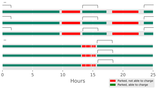
Fig. 6.10 Notional results for immediate charging algorithm, with charging hours within the bracket
Smart charging refers to coordinated charging, where drivers provide information on their travel schedule and charging demand to the electric grid operator.
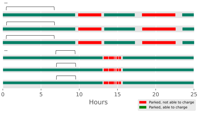
Fig. 6.11 Notional results for smart charging algorithm, with charging hours within the bracket
Example Output – Immediate Charging. Immediate Charging refers to full power charging at time of plug-in until the battery is full or until the vehicle departs on the next driving trip. Fig. 6.12 presents a normalized, unscaled LDV charging demand alongside a normalization of the underlying non-transportation base demand (note: the normalization of the charging profile uses the sum of a full year of charging from the sample vehicles as the denominator). Notice how the uncoordinated charging pattern aligns with the underlying non-transportation base demand.
From there, this normalized profile is then scaled based on the parameters for the desired simulation year, with an example output shown in Fig. 6.1. These parameters include the projected VMT for the simulated year, the fuel efficiency projection (e.g. number of kWh consumed per mile traveled), and the efficiency of the charging process. Notice that the peak demand increases due to the uncoordinated charging pattern.
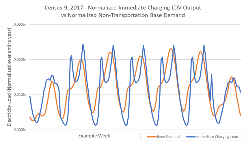
Fig. 6.12 Normalized LDV Immediate Charging output for 1 example week
Example Output – Smart Charging. Smart charging refers to coordinated charging, where drivers provide information on their travel schedule and charging demand to the electric grid operator. Vehicle charging is optimized based on cost (e.g., time-of-use rates), grid support needs, travel considerations, and vehicle constraints. Fig. 6.13 presents a normalized, unscaled LDV smart charging demand alongside a normalization of the underlying non-transportation base demand. Notice how in this case the smart charging pattern no longer aligns with the underlying non-transportation base demand. Fig. 6.2 shows an example of the results from LDV smart charging at scale that was optimized for grid support needs by flattening net demand (e.g. “filling in the valleys”).
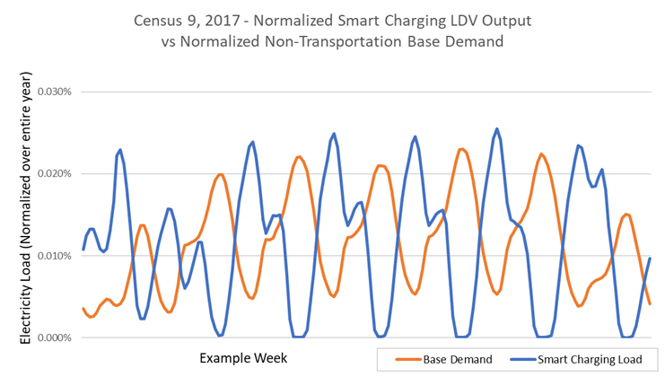
Fig. 6.13 Normalized LDV Smart Charging output for 1 example week
6.2.2.4.2. Vehicle Travel Patterns
6.2.2.4.2.1. Light-duty Travel patterns
The 2017 National Household Travel Survey (NHTS) documents the light-duty vehicle and
light-duty truck travel patterns (https://nhts.ornl.gov/). Data from the NHTS 2017
trippub.csv dataset were filtered to identify all vehicle trips. Relevant data were
then divided into nine datasets, one for each Census Division, as defined within the
dataset, see Table 6.1.
Division Number |
Name |
States Included |
|---|---|---|
01 |
New England |
CT, MA, ME, NH, RI, VT |
02 |
Middle Atlantic |
PA, NJ, NY |
03 |
East North Central |
IL, IN, MI, OH, WI |
04 |
West North Central |
IA, KS, MN, MO, ND, NE, SD |
05 |
South Atlantic |
DE, FL, GA, MD, NC, SC, VA, WV, (DC) |
06 |
East South Central |
AL, KY, MS, TN |
07 |
West South Central |
AR, LA, OK, TX |
08 |
Mountain |
AZ, CO, ID, MT, NM, NV, UT, WY |
09 |
Pacific |
AK, CA, HI, OR, WA |
The definition for each column in the final datasets is in Table 6.2. Columns 1-20 are taken directly from the NHTS dataset, and columns 21-28 are calculated values based on the preceding columns.
Column |
Variable |
|---|---|
1 |
Household |
2 |
Vehicle ID |
3 |
Person ID |
4 |
Scaling Factor Applied |
5 |
Trip Number |
6 |
Date (YYYYMM) |
7 |
Day of Week (1 - 7) |
8 |
If Weekend |
9 |
Trip Start Time (HHMM) |
10 |
Trip End Time (HHMM) |
11 |
Travel Minutes |
12 |
Dwell Time |
13 |
Miles Traveled |
14 |
Vehicle Miles Traveled |
15 |
Why From |
16 |
Why To |
17 |
Vehicle Type (1-4 LDV, 5+ LDT) |
18 |
Household Vehicle Count |
19 |
Household Size |
20 |
Trip Type |
21 |
Start Time (hour decimal) |
22 |
End Time (hour decimal) |
23 |
Dwell Time (hour decimal) |
24 |
Travel Time (hour decimal) |
25 |
Vehicle Speed (mi/hour) |
26 |
Sample Vehicle Number |
27 |
Total Vehicle Trips |
28 |
Total Vehicle Miles Traveled |
Total vehicle trips variable refers to the total number of trips a single vehicle takes in the sample window (24 hours). Trips are divided into weekday and weekend trips. The resulting charging profile for each day type is replicated across the year, i.e., each weekday and each weekend are the same set of trips across the year. Table 6.3 presents the total number of trips in the trip datasets for each vehicle category. The weekday and weekend trips are weighted based on the MOVES weight factors. The charging demand is scaled up and down further based on the MOVES monthly weight factors depending on the month of the year.
Vehicle Category |
Census Division |
Trip Count |
|
|---|---|---|---|
Weekday |
Weekend |
||
LDV |
01 |
3979 |
1235 |
02 |
32831 |
10664 |
|
03 |
30815 |
5116 |
|
04 |
8962 |
2885 |
|
05 |
58173 |
9620 |
|
06 |
2294 |
611 |
|
07 |
52982 |
7818 |
|
08 |
9127 |
2033 |
|
09 |
53554 |
16386 |
|
LDT |
01 |
2881 |
935 |
02 |
29513 |
9347 |
|
03 |
31788 |
5478 |
|
04 |
10157 |
2960 |
|
05 |
58900 |
9465 |
|
06 |
2416 |
678 |
|
07 |
60929 |
8530 |
|
08 |
10006 |
2084 |
|
09 |
40161 |
12116 |
|
MDV |
All |
8302 |
same |
HDV |
All |
8407 |
same |
6.2.2.4.2.2. Medium- and Heavy-duty Vehicles
The construction of the original representative datasets is described in [5].
The following is a description of the data that are rendered from the initial, representative HDV dataset.
Trip times, trip count, and miles traveled – data on trips was taken from the original trip datasets and scaled to align with known statistics for the target region. Only trip count, times, and miles traveled were included. Information on locations, vehicle identity, vehicle class, and vocation are excluded.
Dwell location – dwell locations are simplified to being either a “home base location” or not. Home base locations are defined as depots that are owned, managed, and/or under contract with the same entity as the fleet vehicle.
Trip start and stop times – travel and dwell times by time of day.
The final data table structure is presented in Table 6.4. Each row of the data table is a unique trip taken by the specified vehicle.
Column |
Variable |
Description |
|---|---|---|
1 |
Vehicle Number |
Unique vehicle number |
2 |
Trip Number |
Current trip number of vehicle |
3 |
Destination (home base or not) |
Where the trip ends, 1 = home base, 2 = not home base |
4 |
Trip Distance |
Miles traveled in the trip |
5 |
Trip Start |
Time of trip start |
6 |
Trip End |
Time of trip end |
7 |
Dwell Time |
Length of time vehicle parked between trips |
8 |
Trip Time |
Length of travel time |
9 |
Total Vehicle Trips |
Total count of trips taken by the identified vehicle in the time window |
10 |
Total Vehicle Miles |
Total vehicle miles traveled by vehicle in time window |
6.2.2.4.3. Annual Vehicle Miles Traveled
The model is structured for a single base year (2017) and 33 future years (2018-2050). Each year is unique based on vehicle miles traveled (VMT) and fuel economy (miles per gallon of gasoline equivalent, mi/GGE), which together determine annual vehicle electricity demand. The base year and future projections of battery electric vehicle miles traveled are taken from NREL’s EFS [4]. BEV VMT is divided into VMT occurring in UAs and RAs. UA is a term assigned by the U.S. Census Bureau and is described as areas with a population of 50,000 people or more [2]. Other years are available from NREL, if desired.
6.2.2.4.3.1. Electric Vehicle Miles Traveled Projections by Urban and Rural Area
VMT per capita for each state and UA was taken from the Department of Transportation’s transportation health tool [1]. To determine total state VMT, state population was taken from Census data and was multiplied by the above state VMT per capita data [1] [2]. Then, to calculate the fraction of total state VMT that is allocated to each UA and RA, the UA population was also pulled from Census data [2]. From there, the UA population was multiplied by UA VMT per capita to get total UA VMT. Lastly, UA VMT is subtracted from state VMT to determine the RA VMT for the state. These calculations are summarized below:
6.2.2.4.3.2. Monthly and Daily Weight Factors
Along with the rural/urban distribution, the default scenarios also use weekday/weekend and monthly weight factors to distribute annual VMT. These weight factors come directly from the U.S. EPA’s MOVES model [3]. The weight factor values are listed in Table 6.5 and Table 6.6.
Day Type |
Rural |
Urban |
|---|---|---|
Weekday (divided over 5 days) |
0.72118 |
0.762365 |
Weekend (divided over 2 days) |
0.27882 |
0.237635 |
Month |
Weight Factor |
|---|---|
January |
0.0731 |
February |
0.0697 |
March |
0.0817 |
April |
0.0823 |
May |
0.0875 |
June |
0.0883 |
July |
0.0923 |
August |
0.0934 |
September |
0.0847 |
October |
0.0865 |
November |
0.0802 |
December |
0.0802 |
6.2.2.4.3.3. BEV VMT Projections
To calculate the BEV VMT by vehicle class for each UA, state-level BEV VMT projections were based on NREL’s EFS for 8 vehicle types [4]:
LDV BEV Cars: 100 mi, 200 mi, 300 mi
LDV BEV Trucks: 100 mi, 200 mi, 300 mi
MDV Trucks
HDV Trucks
Projections were used for 2018-2050. The 2017 base year assumptions were calibrated based on historical data. For all years, BEV VMT at the state level was translated to BEV VMT at the UA level by multiplying the state-level projections by the fraction of state VMT allocated to each UA. It is assumed that the proportion of VMT occurring in urban areas relative to total state VMT will be constant moving into the future. There are some UAs that did not have VMT data. Out of 481 UAs, 56 did not have VMT per capita data from the DOT, so those entries will use their respective state’s VMT per capita.
Once each UA and the state’s RA have their projected annual VMT for a simulation year, the annual VMT is distributed to each day of the year based on weight factors from U.S. EPA MOVES model, see Table 6.7. Each daily weight factor represents the fraction of annual VMT that is traveled in that specific day. The daily weight factors vary by month, whether the VMT is in a UA or a RA, and whether the day is a weekday or a weekend day. For example, within a given urban area all weekdays in January have the same weight factor and therefore the same allocated VMT.
Urban |
Rural |
|||
|---|---|---|---|---|
Month |
Weekday |
Weekend |
Weekday |
Weekend |
January |
0.00252 |
0.00196 |
0.00238 |
0.00230 |
February |
0.00266 |
0.00207 |
0.00251 |
0.00243 |
March |
0.00279 |
0.00218 |
0.00266 |
0.00257 |
April |
0.00296 |
0.00231 |
0.00268 |
0.00277 |
May |
0.00299 |
0.00233 |
0.00285 |
0.00275 |
June |
0.00313 |
0.00244 |
0.00297 |
0.00287 |
July |
0.00321 |
0.00250 |
0.00301 |
0.00291 |
August |
0.00319 |
0.00249 |
0.00304 |
0.00294 |
September |
0.00302 |
0.00236 |
0.00285 |
0.00276 |
October |
0.00298 |
0.00232 |
0.00282 |
0.00272 |
November |
0.00284 |
0.00221 |
0.00270 |
0.00261 |
December |
0.00279 |
0.00217 |
0.00262 |
0.00253 |
The trip data are scaled based on the allocated daily VMT. The daily patterns are adjusted by scaling the VMT of each trip within the daily patterns so that the total across the simulation matches the Annual VMT projection for each state.
6.2.2.4.3.4. Fuel Efficiency Projections
NREL’s Electrification Futures Study also projects average BEV fuel economy over time, based on assumptions regarding technology improvements and vehicle range [6]. NREL provides a range of possible BEV fuel economies (“Slow Advancement”, “Moderate Advancement”, and “Rapid Advancement”). The charging model uses the “Moderate Advancement” values as the default fuel economy for each vehicle category and year, as shown in Table 6.8.
Vehicle Type |
Fuel Economy (mile/GGE) |
||||
|---|---|---|---|---|---|
2017-2019 |
2020-2024 |
2025-2034 |
2035-2044 |
2045-2050 |
|
LDV BEV cars, 100 mile range |
103 |
117 |
137 |
153 |
159 |
LDV BEV cars, 200 mile range |
97 |
112 |
133 |
149 |
155 |
LDV BEV cars, 300 mile range |
85 |
102 |
124 |
138 |
144 |
LDT BEV trucks, 100 mile range |
60 |
69 |
78 |
83 |
85 |
LDT BEV trucks, 200 mile range |
57 |
66 |
76 |
81 |
83 |
LDT BEV trucks, 300 mile range |
50 |
60 |
72 |
76 |
79 |
MDV trucks |
16 |
17 |
19 |
21 |
22 |
HDV trucks |
9 |
10 |
13 |
14 |
15 |
6.2.2.4.4. Smart Charging Optimization Algorithm
The smart charging algorithm was developed by [7]. The algorithm is a least cost optimization problem, with the cost function as follows:
The total number of dwell segments \(seg(i)\) will depend on the how long the vehicle is parked.
Equality constraint:
Inequality constraints:
Bounds:
The optimization is structured to minimize the cost to charge each battery electric vehicle within defined battery constraints. It is conducted at hourly timescale, meaning that cost and electricity demand are provided in hourly segments. Charging efficiency is dependent on the type of electric vehicle supply equipment (EVSE). Efficiency tends to increase with higher charging rates. The model currently distinguishes between the lower charging efficiency of AC level 2 charging (90%) and DC charging (95%), where AC charging is assumed for charging rates at or below 19.2 kW, and DC charging is assumed for charging rates above 19.2 kW. If a dwell time (\(\Delta t\)) falls below one hour, the charge (\(x\)) available for that segment will be reduced proportional to the amount of time spent parked (i.e., if a vehicle is parked for 30 minutes, the charge will be reduced to \(1/2\)). The default minimum dwell time to consider a charging event is 0.2 hours, or 12 minutes. This value can be modified depending on the user’s scenario. The minimum dwell time is set in order to avoid impractical charging events where, in the real world, a vehicle operator would not plug in their vehicle due to the shortness of the stop. If the charging rate available is high (e.g., DC Fast Charging), a shorter minimum dwell time may be warranted.
6.2.2.4.5. Adoption Rate
As discussed in Section 6.2.2.4.3.3, the default BEV adoption rates used in this model are the VMT projections from NREL’s EFS data. NREL used their Automotive Deployment Options Projection Tool (ADOPT) in 2017 to generate the 2018-2050 projections. Once actual adoption rates become available, those values could be used at the state and/or UA level to update all remaining VMT projections. As an example, the California Energy Commission publishes a dashboard of the Light Duty Vehicle Population by fuel type (including BEVs) in California for past years.
Similarly, other updates of BEV adoption rate projections at both state and UA levels undoubtedly will arise over time. As discussed in the User Manual section above, using the user interface and modifying the accompanying datasets would allow updated adoption rate projections to create corresponding BEV charging profiles when desired. Links for these data sources are available in Section 6.2.2.5.
6.2.2.5. Data Sources
The detailed data sets are developed using data from the following sources:
National Household Travel Survey (NHTS) from 2017 documents the light-duty vehicle and light-duty truck travel patterns: https://nhts.ornl.gov
US Department of Transportation, Transportation and Health Indicators: https://www7.transportation.gov/transportation-health-tool/indicators
United States Census Bureau, 2010 Census Urban and Rural Classification and Urban Area Criteria: https://www.census.gov/programs-surveys/geography/guidance/geo-areas/urban-rural/2010-urban-rural.html
National Renewable Energy Laboratory, Electric Technology Adoption and Energy Consumption | NREL Data Catalog: https://data.nrel.gov/submissions/92
P. Jadun, C. McMillan, D. Steinberg, M. Muratori, L. Vimmerstedt, and T. Mai, Electrification Futures Study: End-Use Electric Technology Cost and Performance Projections through 2050: https://www.nrel.gov/docs/fy18osti/70485.pdf
U.S. Environmental Protection Agency, MOVES and Other Mobile Source Emissions Models: https://www.epa.gov/moves
NREL’s Automotive Deployment Options Projection Tool (ADOPT): https://www.nrel.gov/transportation/adopt.html
California Energy Commission’s Light-Duty Vehicle Population in California: https://www.energy.ca.gov/data-reports/energy-almanac/zero-emission-vehicle-and-infrastructure-statistics/light-duty-vehicle
University of California’s Institute of Transportation Studies Report: Driving California’s Transportation Emissions to Zero. https://escholarship.org/uc/item/3np3p2t0
EMFAC’s https://arb.ca.gov/emfac/emissions-inventory/0e7a83330a66b634f8c81b376ab6696cbd42e113
6.2.3. NREL Electrification Futures Study Demand and Flexibility Data
The National Renewable Energy Laboratory (NREL) has developed the Electrification Futures Study (EFS) to project and study future sectoral demand changes as a result of impending widespread electrification. As a part of the EFS, NREL has published multiple reports (dating back to 2017) that describe their process for projecting demand-side growth and provide analysis of their preliminary results; all of NREL’s published EFS reports can be found here. Accompanying their reports, NREL has published data sets that include hourly load profiles that were developed using processes described in the EFS reports. These hourly load profiles represent state-by-state end-use electricity demand across four sectors (Transportation, Residential Buildings, Commercial Buildings, and Industry) for three electrification scenarios (Reference, Medium, and High) and three levels of technology advancements (Slow, Moderate, and Rapid). Load profiles are provided for six separate years: 2018, 2020, 2024, 2030, 2040, and 2050. The base demand data sets and further accompanying information can be found here. In addition to demand growth projections, NREL has also published data sets that include hourly profiles for flexible load. These data sets indicate the amount of demand that is considered to be flexible, as determined through the EFS. The flexibility demand profiles consider two scenarios of flexibility (Base and Enhanced), in addition to the classifications for each sector, electrification scenario, technology advancement, and year. The flexible demand data sets and further accompanying information can be found here.
Widespread electrification can have a large impact on future power system planning decisions and operation. While increased electricity demand can have obvious implications for generation and transmission capacity planning, new electrified demand (e.g., electric vehicles, air source heat pumps, and heat pump water heaters) offers large amounts of potential operational flexibility to grid operators. This flexibility by demand-side resources can result in demand shifting from times of peak demand to times of peak renewable generation, presenting the opportunity to defer generation and transmission capacity upgrades. To help electrification impacts be considered properly, this package has the ability to access NREL’s EFS demand data sets. Currently, users can access the base demand profiles, allowing the impacts of demand growth due to vast electrification to be explored. Users can also access the EFS flexible demand profiles.
The NREL EFS demand notebook and NREL EFS flexibility notebook, illustrate the functionality of the various modules developed for obtaining and cleaning the NREL’s EFS demand data.
6.3. Hydro
6.3.1. Texas
ERCOT publishes actual generation by fuel type for each 15 minute settlement interval (see the fuel mix report for more details). The profile of each hydro plant in the Texas Interconnection is then simply the ratio of the total generation provided by ERCOT divided by the total hydro capacity available in the Texas Interconnection of the grid model.
The texas hydro notebook generates the profile.
6.3.2. Western
Unlike Texas, we don’t have access to hourly (or sub-hourly) total generation by state or even for the whole Western Interconnection. We rely on three different methods to derive the shape of the hydro profile in California, Wyoming and the rest of the Western Interconnection.
California: we use the net demand profile as a template. This is supported by data from California ISO (see CAISO outlook) showing that the hydro generation profile closely follows the net demand profile.
Wyoming: we simply apply a constant shape curve to avoid peak-hour violation of maximum capacity since hydro generators have a small name plate capacities.
other region in the Western Interconnection: we use the aggregated generation of the top 20 US Army Corps managed hydro dams in Northwestern US (primarily located in the state of Washington) as the shape of the hydro profile since WA has the most hydro generation in the Western Interconnection. The data is obtained via the US Army Corps of Engineers Northwestern Division DataQuery Tool 2.0 (see USACE dataquery).
The above curves are then normalized such that the monthly sum in each of the above regions is equal to the total monthly hydro generation divided by the total hydro capacity available in the grid model for the region. Note that EIA form 923 provides the historical monthly total hydro generation by state.
The western hydro notebook generates the profile.
6.3.3. Eastern
Profile generation for the Eastern Interconnection is slightly more complex than for the Western Interconnection. First, we handle pumped storage hydro (HPS) and conventional hydro (HYC) separately. Then, in addition to using the net demand profile to derive the profile of conventional hydro plants in some state as we did for California, we also use historical hourly total hydro generation time series in some regions.
Pumped Storage Hydro: We identified hydro plants in our grid model that are closely located to known HPS site in the Eastern Interconnection and created a template to describe the hourly energy generation. The plant level profile is generated considering the local time and daylight-saving schedule of the corresponding bus location.
Conventional hydro: profiles provided by ISONE, NYISO, PJM and SPP are used for plants located within the area they cover. For states that are not at all covered or partially covered by the 4 ISOs the net demand demand is used as a template to derive the hydro profile using the same method that has been developed for California, i.e., the monthly net demand is normalized such that its sum is equal to the historical monthly total hydro generation (reported in EIA form 923) divided by the available total hydro capacity in the grid model. Note that for partially covered states, the historical monthly total hydro generation in the state is split proportionally to the available total hydro capacity in the grid model for the state and only the portion outside the ISOs is used during the normalization.
The eastern hydro notebook generates the profile.
6.4. Renewables
6.4.1. Solar
6.4.1.1. The National Solar Radiation Database
The National Solar Radiation Database (NSRDB) provides 1-hour resolution solar radiation data, ranging from 1998 to 2017, for the entire U.S. and a growing list of international locations on a 4x4 square kilometer grid. The Physical Solar Model (PSM) v3 is the version of the NSRDB used.
An API can be used to fetch the data. A key is required to access and use the above databases. Get your own API key here.
6.4.1.2. From Solar Irradiance to Power Output
6.4.1.2.1. Naive
Power output is estimated using a simple normalization procedure. For each solar plant location in the grid model the hourly Global Horizontal Irradiance (GHI) is divided by the maximum GHI over the period considered. This procedure is referred to as naive since other factors can possibly affect the conversion from solar radiation at ground to power such as the temperature at the site as well as many system configuration including tracking technology.
6.4.1.2.2. System Adviser Model
The System Adviser Model (SAM) developed by NREL is used to estimate the power output of a solar plant. Irradiance data along with other meteorological parameters must first be retrieved from NSRDB for each plant site. This information is then fed to the SAM Simulation Core (SCC) and the power output is retrieved. The PySAM Python package provides a wrapper around the SAM library. The PVWatts v7 model is used for all the solar plants in the grid. The system size (in DC units) and the array type (fixed open rack, backtracked, 1-axis and 2-axis) is set for each solar plant whereas a unique value of 1.25 is used for the DC to AC ratio (see article from EIA on inverter loading ratios). Otherwise, all other input parameters of the PVWatts model are set to their default values. EIA form 860 reports the array type used by each solar PV plant. For each solar plant in our network, the array type is a combination of the three technology and calculated via the capacity weighted average of the array type of all the plants in the EIA form that are located in the same state. If no solar plants are reported in the form for a particular state, we then consider plants belonging to the same interconnect.
6.4.2. Wind
6.4.2.1. Rapid Refresh
RAP (Rapid Refresh) is the continental-scale NOAA hourly-updated assimilation/modeling system operational at the National Centers for Environmental Prediction (NCEP). RAP covers North America and is comprised primarily of a numerical weather model and an analysis system to initialize that model. RAP provides for every hour ranging from May 2012 to date, the U and V components of the wind speed at 80 meter above ground on a 13x13 square kilometer resolution grid every hour. Data can be retrieved using the NetCDF Subset Service.
6.4.2.2. High-Resolution Rapid Refresh
The HRRR (High-Resolution Rapid Refresh) is a NOAA real-time 3-km resolution, hourly updated, cloud-resolving, convection-allowing atmospheric model, initialized by 3km grids with 3km radar assimilation. Radar data is assimilated in the HRRR every 15 min over a 1-h period adding further detail to that provided by the hourly data assimilation from the 13km radar-enhanced Rapid Refresh. Data can be retrieved from a publicly available AWS S3 Bucket.
6.4.2.3. From Wind Speed to Power Output
Once the U and V components of the wind are converted to a non-directional wind speed magnitude, this speed is converted to power using wind turbine power curves. Since real wind farms are not currently mapped to a grid network farms, a capacity-weighted average wind turbine power curve is created for each state based on the turbine types reported in EIA Form 860. The wind turbine curve for each real wind farm is looked up from a database of curves (or the IEC class 2 power curve provided by NREL in the WIND documentation is used for turbines without curves in the database), and scaled from the real hub heights to 80m hub heights using an alpha of 0.15. These height-scaled, turbine-specific curves are averaged to obtain a state curve translating wind speed to normalized power. States without wind farms in EIA Form 860 are represented by the IEC class 2 power curve.
Each turbine curve represents the instantaneous power from a single turbine for a given wind speed. To account for spatio-temporal variations in wind speed (i.e. an hourly average wind speed that varies through the hour, and a point-specific wind speed that varies throughout the wind farm), a distribution is used: a normal distribution with standard deviation of 40% of the average wind speed. This distribution tends to boost the power produced at lower wind speeds (since the power curve in this region is convex) and lower the power produced at higher wind speeds (since the power curve in this region is concave as the turbine tops out, and shuts down at higher wind speeds). This tracks with the wind-farm level data shown in NREL’s validation report.
6.4.3. Resources
6.4.4. Command Line Interface
Wind and solar data can be downloaded via our download manager python script. When in the terminal at the project root directory, you can run:
python -m prereise.cli.download.download_manager -h
usage: download_manager.py [-h] {wind_data_rap,solar_data_ga,solar_data_nsrdb} ...

positional arguments:
  {wind_data_rap,solar_data_ga,solar_data_nsrdb}
    wind_data_rap       Download wind data from National Centers for Environmental Prediction
    solar_data_ga       Download solar data from the Gridded Atmospheric Wind Integration National Dataset Toolkit
    solar_data_nsrdb    Download solar data from the National Solar Radiation Database

optional arguments:
-h, --help            show this help message and exit
Currently supported data sources to download from are:
Rapid Refresh from National Centers for Environmental Prediction:
python -m prereise.cli.download.download_manager wind_data_rap \
--region REGION \
--start_date START_DATE \
--end_date END_DATE \
--file_path FILEPATH
Gridded Atmospheric Wind Integration National Dataset Toolkit:
python -m prereise.cli.download.download_manager solar_data_ga \
    --region REGION \
    --start_date START_DATE \
    --end_date END_DATE \
    --file_path FILEPATH \
    --key API_KEY
The National Solar Radiation Database:
python -m prereise.cli.download.download_manager solar_data_nsrdb \
    --region REGION \
    --method METHOD \
    --year YEAR \
    --file_path FILEPATH \
    --email EMAIL \
    --key API_KEY
As a concrete example, if you would like to download the wind data from Rapid Refresh
from National Centers for Environmental Prediction for the Texas and Western
interconnections between the dates of June 5th, 2020 and January 2nd, 2021 into
data.pkl, you can run:
python -m prereise.cli.download.download_manager wind_data_rap \
--region Texas \
--region Western \
--start_date 2020-05-06 \
--end_date 2021-01-02 \
--file_path ./data.pkl
Note that missing data, if existing, will be imputed using a naive Gaussian algorithm.
This can be avoided using the --no_impute flag.
6.4.5. Notebooks
The RAP notebook fetches the data, imputes missing data and generates a profile.
The NSRDB SAM notebook generates a solar profile by feeding the NSRDB data to SAM while the NSRDB naive notebook uses the naive method.
The GA WIND naive notebook generates solar profiles by applying the naive method to the Gridded Atmospheric Wind Integration National Dataset.
6.4.6. Bibliography
US Department of Transportation. Transportation and health indicators. https://www7.transportation.gov/transportation-health-tool/indicators. Accessed Jun. 21, 2022.
US Census Bureau. 2010 census urban and rural classification and urban area criteria. https://www.census.gov/programs-surveys/geography/guidance/geo-areas/urban-rural/2010-urban-rural.html. Accessed Jun. 21, 2022.
US Environmental Protection Agency. Moves and other mobile source emissions models. https://www.epa.gov/moves. Accessed Jun. 21, 2022.
US Census Bureau. Electric technology adoption and energy consumption | nrel data catalog. https://data.nrel.gov/submissions/92. Accessed Jun. 21, 2022.
B. Tarroja K. Forest, M. Mac Kinnon and S. Samuelsen. Estimating the technical feasibility of fuel cell and battery electric vehicles for the medium and heavy duty sectors in california. Applied Energy, 276:115439, 2020. URL: https://www.sciencedirect.com/science/article/pii/S030626192030951X, doi:https://doi.org/10.1016/j.apenergy.2020.115439.
P. Jadun et al. Electrification Futures Study: End-Use Electric Technology Cost and Performance Projections through 2050. National Renewable Energy Laboratory, Golden, CO: National Renewable Energy Laboratory. NREL/TP-6A20-70485. Accessed April 2, 2018.
L. Zhang. Charging infrastructure optimization for plug-in electric vehicles. PhD thesis, UC Irvine, 2014. Retrieved from https://escholarship.org/uc/item/0199j451, Accessed June 21, 2017.
